[Leveraged Finance] Expected Return and Risk
Leveraged loans attract investors and asset allocators based on three key features: seniority, security/collateral, and the floating rate nature of loan returns. The first two components mitigate credit risk, and the third virtually eliminates interest rate risk.
Leveraged loans are not securities. This fundamental characterization makes it private credit, in contrast to public credit such as high-yield bonds. Therefore, investors must assess private credit investment relative to other asset classes before deciding its desirable allocation within an overall portfolio. This post describes the capital market assumptions on risk and return of different asset classes. A theoretical framework is also introduced to tackle credit pricing.
Expected Return and Risk: Private Credit vs Other Asset Classes
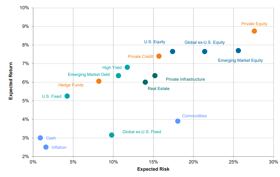
For institutional investors, one of key inputs to determine the asset allocation is long-term reutrn and risk for individual asset classes. Below is the 2024-2033 capital market assumptions from Callan, an investment consulting firm. Their calculation indicates Private Credit would earn 7.4%, slightly higher than High Yied bond as compensation for illiquidity and complexity
Expected Return Calculation: Private Credit - Corporate Lending
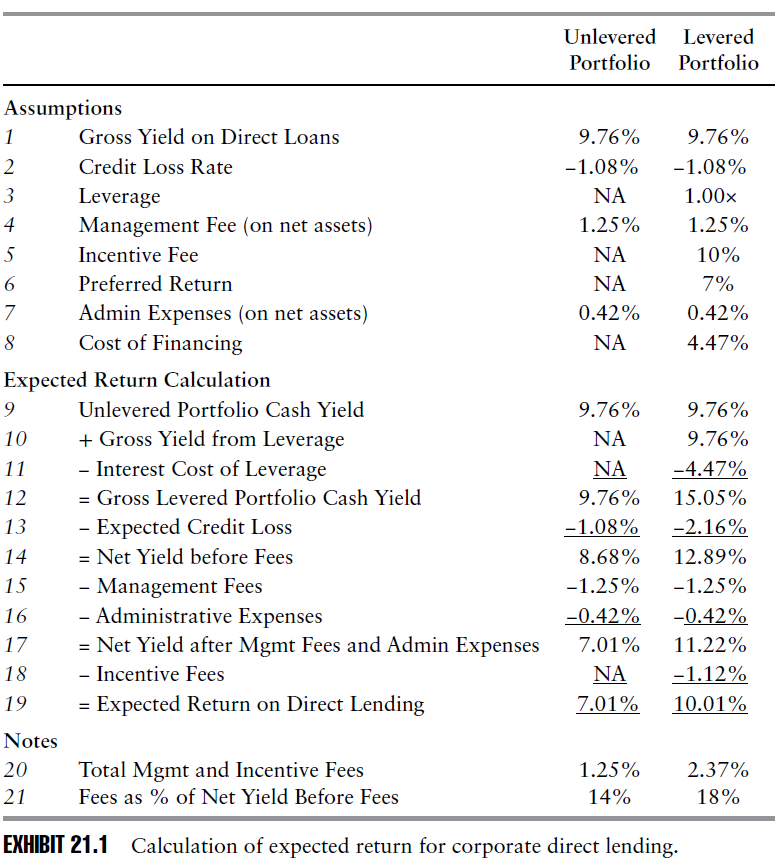
Nesbitt [1] provides an illustrative calculation for ten-year return forecasts for corporate lending based on eight key assumptions.
- Gross Yield (Line 1) and Credit Loss Rate (Line 2) are two critical inputs that are estimates and hence subject to uncertainty.
- Leverage (Line 3) and Cost of Finance (Line 8) are equally important when leverage is used to enhance return.
Merton's Option Theory for Credit
In Merton's world, the accounting equation and the put-call parity are married to birth a popular corporate credit theory.
- Accounting: Asset = Equity + Liabilities
- Put-Call Parity: Call - Put = Discount * (Forward Price of Asset - Strike Price)
Specifically, Equity investors / Shareholders pay some price to have a claim on the residual interest in the firm's assets after deducting liabilities. Shareholders can be thought of buying a call option. In the same spirit, Corporate lenders / Creditors sell a put option, receive a credit risk premium, and expect full repayment at maturity plus interest. For example, buy an AAA-graded (or B-graded) bond with a face value of $100 at $98 (or $90).
$$ \begin{align*} \text{Discount} * \text{Forward Price of Asset} &= \text{Call} &+ \text{Discount} * \text{Strike Price} - \text{Put} \ \text{Market Value of Asset} &= \text{Market Cap of Equity} &+ \text{Total Liabilities} - \text{Credit Risk Premium} \ \end{align*} $$
With this insight, the Black-Scholes formula is easily applicable for estimating gross yield and credit loss rate.
- gross yield = risk-free rate + credit risk premium
- credit loss rate = PD * EAD * LGD
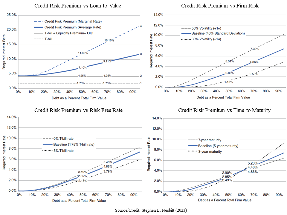
Per theory, credit risk premium responds to four risk factors; LTV, asset vol, risk-free interest, and time-to-maturity. Among others, the Debt-to-Asset ratio and asset volatility are particularly important in estimating the default probability. Distance-to-Default (DD), for instance, calculates the difference between asset and default point (e.g., current liability + 1/2 LT liability), scaled by unobservable asset volatility, and maps it to a probability value from [0, 1] via certain measurement (e.g., logistic function).
Empirically, loans are announced with a target price, but the actual price will either flex up or flex down depending on demand and general market conditions. The targeted price is negotiated and agreed by arrangers (e.g., bank) and issuer/borrower, at the time the mandate to lead the loan was granted. This is in contrast to bonds, which are typically priced when the offering is completed, based on the pricing required to "clear the market" and sell the entire issue. Therefore, loans need the inclusion of pricing "flex" to resemble that of bonds. Below are a few examples
- IB executed the reprice tight of talk, reducing the spread from S+300 bps to S+250 bps while removing the credit spread adjustment ("CSA"), achieving 75 bps of interest savings for the firm
- IB's execution resulted in final pricing of S+300 bps | 99.75 OID; compared to price talk of S+350-375 bps | 99.50 OID.
Still, the theory remains useful in 1) guiding the target price and 2) estimating the real-time credit loss rate, two of which can shed light on a reasonable expected return on credit investment.
Reference
[1] Stephen L. Nesbitt, 2023, Private Debt: Yield, Safety and the Emergence of Alternative Lending